Using random forest to predict bandgaps and HOMOs

A new idea that we can bypass quantum chemistry calculation using the proper machine learning method is prevalent now. It will be exciting if we could have a second way to resolve objectives of material discovery quest rather than adopting Density functional theory (DFT) that is the principal method used now. Here I will primarily compare predictions from DFT and a popular machine learning method called the Random Forest (RF). The objective is to predict the bandgaps and HOMOs (highest occupied molecular orbitals) energies of organic semiconductors.

Molecular fingerprint

The molecular fingerprint is a method to digitize the features of a molecule into a binary code. Depending on the specific scheme, there are several ways to do that. The one that used to be popular is MACCS that was developed by MDL as a drug screening tool to select molecules with a similar structure. The public version has 166 binary bits, and each bit takes specific value if the molecule has a particular feature.

However, the fingerprint scheme that we are going to use is Morgan fingerprint (circular fingerprint). Compared to other fingerprints, Morgan includes features like the number of Pi electron and other electronic related properties:

Morgan describes the local environment and the connectivity of each atom within certain radius, e.g. Morgan2 means coding the environment and connectivity within r=2.
Features defined in Morgan include: numbers of Pi electrons, electronic donor property or acceptor property.

Since our goal is to predict the bandgap of organic molecules whose energy level are mostly decided by n electrons (n->Pi: infrared band) or Pi electrons (Pi->Pi: UV-Vis band ), all of which have something to do with electronic property, so I feel Morgan is appropriate to use. However, other fingerprints may also be choices, since features like topology also determined by the electronic property of the molecules, although not so directly.

Using the python library RDkit and Jupyter notebook, we can visualize some of the features that Morgan encoded:

( You can also run the following source code on google colab: https://colab.research.google.com/drive/1vaL9XrL0MVOlo4yBIKeZ8deavvO-51FF )

from rdkit import Chem
from rdkit.Chem import rdMolDescriptors
from rdkit.Chem import Draw
from rdkit.Chem.Draw import IPythonConsole

# First load the molecule
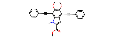
mymol_M8f=Chem.MolFromSmiles('COC(=O)C1=CC2=C(C#CC3=CC=CC=C3)C(=C(OC)C(=C2[N]1C)C#CC4=CC=CC=C4)OC')
mymol_M8f

# Calculate Morgan Fingerprint and show features encoded:
bi_M8f = {}
Morgan_fp_M8f = rdMolDescriptors.GetMorganFingerprintAsBitVect(mymol_M8f, radius=2, bitInfo=bi_M8f)
print(bi_M8f)
{56: ((8, 2), (24, 2)), 102: ((10, 1), (26, 1)), 145: ((2, 1),), 189: ((9, 2), (25, 2)), 213: ((7, 1), (20, 1)), 236: ((7, 2),), 333: ((17, 1), (16, 1)), 342: ((6, 2),), 389: ((13, 2), (29, 2)), 430: ((8, 1), (9, 1), (24, 1), (25, 1)), 488: ((4, 1),), 564: ((22, 1),), 609: ((4, 2),), 650: ((3, 0),), 674: ((8, 0), (9, 0), (24, 0), (25, 0)), 695: ((1, 0), (18, 0), (32, 0)), 807: ((2, 0),), 835: ((2, 2),), 841: ((0, 1), (19, 1), (33, 1)), 875: ((5, 1),), 885: ((21, 2),), 906: ((1, 2),), 935: ((22, 0),), 1057: ((0, 0), (19, 0), (23, 0), (33, 0)), 1088: ((12, 1), (13, 1), (14, 1), (28, 1), (29, 1), (30, 1)), 1140: ((10, 2), (26, 2)), 1145: ((23, 1),), 1152: ((1, 1),), 1156: ((17, 2), (16, 2)), 1199: ((12, 2), (28, 2), (14, 2), (30, 2)), 1357: ((6, 1),), 1380: ((4, 0), (6, 0), (7, 0), (10, 0), (16, 0), (17, 0), (20, 0), (21, 0), (26, 0)), 1440: ((21, 1),), 1536: ((18, 1), (32, 1)), 1553: ((22, 2),), 1599: ((18, 2), (32, 2)), 1734: ((11, 2), (15, 2), (27, 2), (31, 2)), 1750: ((11, 1), (27, 1), (15, 1), (31, 1)), 1793: ((20, 2),), 1794: ((5, 2),), 1873: ((5, 0), (11, 0), (12, 0), (13, 0), (14, 0), (15, 0), (27, 0), (28, 0), (29, 0), (30, 0), (31, 0)), 1917: ((3, 1),)}

The output is a dictionary with bit IDs as keys and (atom ID, radius) as values. For example: 56:((8,2),(24,2)) means this feature (No.56 ) show up at atom8 at radius2 and atom24 at radius2.

We can check what is this feature:

# Draw feature 56
Draw.DrawMorganBit(mymol_M8f,56,bi_M8f)

The blue dot show where is the coordinates origin. Yellow shows the feature. We can also visualize the top 10 features:

# Draw the top 10 features
tpls = [(mymol_M8f,x,bi_M8f) for x in Morgan_fp_M8f.GetOnBits()]
Draw.DrawMorganBits(tpls[:10],molsPerRow=4,legends=[str(x) for x in Morgan_fp_M8f .GetOnBits()][:10])

We can see that they all Pi electron conjugation structures. With the latest RDKit (release 2018.09), you can do more to visualize the features, check their blog post: http://rdkit.blogspot.com/2018/10/using-new-fingerprint-bit-rendering-code.html

In this study, radius=2 and length of bit=1024:

# Morgan: radius=2 and length of bit=1024:
Morgan_fingerprint.append(AllChem.GetMorganFingerprintAsBitVect(mol,2,nBits=1024))

The complete code see: https://github.com/shuod/scripts_for_MachineLearning_projects/tree/master/1_Using%20random%20forest%20to%20predict%20bandgaps%20and%20HOMOs

Another fingerprint I used is RDKit that mostly coded on bond topology.

Random Forest (RF)

When we make a decision, we often encounter a yes-no question: “to be or not to be, that is a question.”. A yes-no question correspond to essentially a binary tree structure, or in this case, it is called a decision tree that is a tree having just two branches(the “yes” branch and the “no” branch). Assuming you are asking your friends for an opinion, “should I pursue her or not?”. One friend may tell you “Yes” after he makes a decision, and the other friend may say “Yes” as well, but the third friend may say “No”. Each of them can be depicted as a decision tree that returns you a decision. Suppose you have a great many friends and each of your friends also has their friends, then your huge “friend network” is made up of a great many decision trees, or we call it the forest.

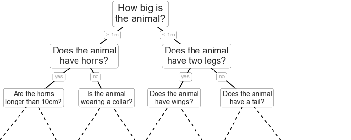
Illustration of random forests and decision trees (from “Python Data Science Handbook, by Jake VanderPlas, O’Reilly Media, 2016” )

If you just look at the hierarchy structure above, it would remind you of the ensemble theory in statistical physics. Indeed, random forest belongs to what is called ensemble learning, because it is an ensemble of decision trees. Also, it looks like the percolation graph, which is a model of particles going through the porous media except now we have one type of particles and the chance of splitting at each node is a fixed value of 50%.

More often than not, we can use three hyper-parameters to tune in order to achieve the best prediction accuracy:

The number of trees or n_estimator (in scikit-learn);
The maximum layers of the trees or max_depth (in scikit-learn);
The maximum number of features to be considered at each split or max_features (in scikit-learn);

However, here I will just optimize the n_estimator(number of trees) since it is computationally affordable to run in my laptop.

Also, there are several parameters to tune the speed: - n_jobs: how many CPU cores to use, “-1” means no restrictions; - random_state: reproduce the same results if given a fixed number; - oob_score: used the CV method in random forest which is faster than generalized CV;

The Random forest can do classification problems as shown in the figure above, and it also can do regression problems. Here we will use it to do a regression to predict bandgap and HOMOs for organic semiconductor.

In this study, I used GridSearchCV() to optimize the n_estimator only:

RF_on_HOMO_Morgan = GridSearchCV(RandomForestRegressor(), cv=8, param_grid={"n_estimators": np.linspace(50, 300, 25).astype('int')},scoring='neg_mean_absolute_error', n_jobs=-1)

The complete code see: https://github.com/shuod/scripts_for_MachineLearning_projects/tree/master/1_Using%20random%20forest%20to%20predict%20bandgaps%20and%20HOMOs